import pandas as pd
import numpy as np
import matplotlib.pyplot as plt
import matplotlib.colors as mcolors
import seaborn as sns
from numpy.linalg import cholesky, qr, cond, lstsq, solve
from scipy.optimize import curve_fit
from sage.all import *
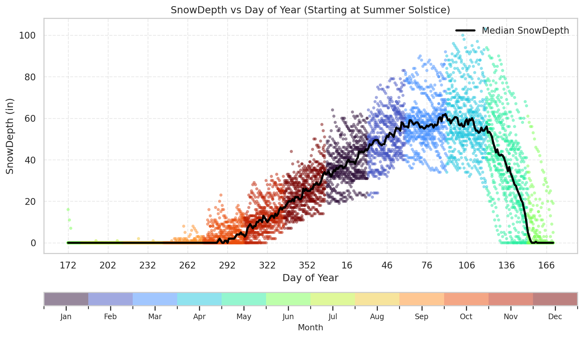
def plot_snowdepth_shifted(df, solstice_day=172, ycol='SnowDepth'):
"""
Plot snow depth vs. rebased day-of-year (starting at summer solstice),
including the median snow depth for each day.
Parameters
----------
df : DataFrame
Input dataset containing 'Date', 'Month', 'DayOfYear', 'SnowDepth',
and 'MedianSnowDepth' columns.
solstice_day : int, optional
Day-of-year for the summer solstice (default 172).
ycol : str, optional
Column name to plot on the y-axis (default 'SnowDepth').
Returns
-------
None
Displays a scatter plot with median line and month colorbar.
"""
work = df.copy()
work['DayShifted'] = (work['DayOfYear'] - solstice_day) % 366
work = work.sort_values('DayShifted')
# Discrete colormap by month
cmap = plt.cm.turbo
month_colors = cmap(np.linspace(0, 1, 12))
norm = mcolors.BoundaryNorm(np.arange(1, 14), 12)
# Plot
plt.figure(figsize=(10, 6))
sc = plt.scatter(work['DayShifted'], work[ycol],
c=work['Month'],
cmap=mcolors.ListedColormap(month_colors),
norm=norm,
s=14, alpha=0.5, edgecolor='none')
# Median Line (using precomputed MedianSnowDepth)
median_by_day = work.groupby('DayShifted')['MedianSnowDepth'].first()
plt.plot(median_by_day.index, median_by_day.values,
color='black', linewidth=2.5,
label='Median {}'.format(ycol))
# Labels and grid
plt.xlabel('Day of Year')
plt.ylabel(ycol + ' (in)')
plt.title('{} vs Day of Year (Starting at Summer Solstice)'.format(ycol))
plt.grid(True, linestyle='--', alpha=0.4)
plt.legend(frameon=False, loc='upper right')
# Horizontal colorbar for months
cbar = plt.colorbar(sc, orientation='horizontal', pad=0.12, aspect=40)
cbar.set_ticks(np.arange(1.5, 13.5))
cbar.set_ticklabels(['Jan','Feb','Mar','Apr','May','Jun',
'Jul','Aug','Sep','Oct','Nov','Dec'])
cbar.ax.tick_params(labelsize=9)
cbar.set_label('Month', fontsize=10)
# X-axis ticks labeled by true day-of-year
xticks = np.arange(0, 366, 30)
plt.xticks(xticks, [str(int((solstice_day + x) % 366)) for x in xticks])
plt.tight_layout()
plt.show()
def add_period(df, name, start, end, col_prefix=None):
"""
Add boolean and day-count columns for a named seasonal period.
Parameters
----------
df : DataFrame
Input dataset with 'Date' and 'DayOfYear' columns.
name : str
Name of the period (e.g., 'Cold', 'Melt').
start, end : int or str
Start and end of the period as day-of-year integers or ISO date strings.
col_prefix : str, optional
Optional column name prefix override.
Returns
-------
DataFrame
Original DataFrame with '<prefix>_InPeriod' and '<prefix>_Day' columns.
"""
prefix = col_prefix or name
# Absolute date mode
if isinstance(start, str) and isinstance(end, str):
start_date = pd.to_datetime(start)
end_date = pd.to_datetime(end)
if end_date >= start_date:
in_period = (df['Date'] >= start_date) & (df['Date'] <= end_date)
day_val = (df['Date'] - start_date).dt.days
else:
in_period = (df['Date'] >= start_date) | (df['Date'] <= end_date)
day_val = ((df['Date'] - start_date).dt.days) % 365
# Day-of-year mode
elif isinstance(start, (int, np.integer)) and isinstance(end, (int, np.integer)):
# Normalize within [1, 365]
start = int(start) % 365 or 365
end = int(end) % 365 or 365
# Inclusive cyclic logic
if start <= end:
in_period = (df['DayOfYear'] >= start) & (df['DayOfYear'] <= end)
day_val = df['DayOfYear'] - start
else:
# Wrap-around case (e.g. 274 -> 90)
in_period = (df['DayOfYear'] >= start) | (df['DayOfYear'] <= end)
# Ensure continuous day count across boundary
day_val = (df['DayOfYear'] - start) % 365
else:
raise ValueError("start and end must both be ints (DayOfYear) or both be strings (absolute dates).")
# Add columns to df
df[f'{prefix}_InPeriod'] = in_period
df[f'{prefix}_Day'] = np.where(in_period, day_val, np.nan)
return df
def get_period_data(df, period_name):
"""
Extract X and y arrays for a given period.
Parameters
----------
df : DataFrame
Dataset with '<Period>_InPeriod' and '<Period>_Day' columns.
period_name : str
Period name (e.g., 'Cold', 'Melt').
Returns
-------
tuple
(X, y, fallback_model) where fallback_model returns NaNs if empty.
"""
in_col = f"{period_name}_InPeriod"
day_col = f"{period_name}_Day"
# Ensure required columns exist
for col in [in_col, day_col, "SnowDepth"]:
if col not in df.columns:
raise KeyError(f"Missing required column '{col}' in DataFrame")
# Subset valid data
df_period = df[df[in_col]].dropna(subset=[day_col, "SnowDepth"])
if df_period.empty:
print(f"No data found for period '{period_name}'")
return None, None, lambda x: np.full_like(np.asarray(x), np.nan, dtype=float)
X = df_period[day_col].values
y = df_period["SnowDepth"].values
return X, y, None
def make_line_model(coeffs, X_mean=0.0):
"""
Create a simple linear model function from coefficients.
Parameters
----------
coeffs : array_like
[intercept, slope]
X_mean : float, optional
Mean of X used for centering (default 0.0)
centered : bool, optional
Whether to subtract X_mean before predicting (default True)
Returns
-------
function
model(x) -> predicted y
"""
a, b = coeffs
return lambda x: a + b * (np.asarray(x, dtype=float) - X_mean)
def plot_period_fits(df, period_name, fit_functions, labels=None,
title=None, show_bands=False):
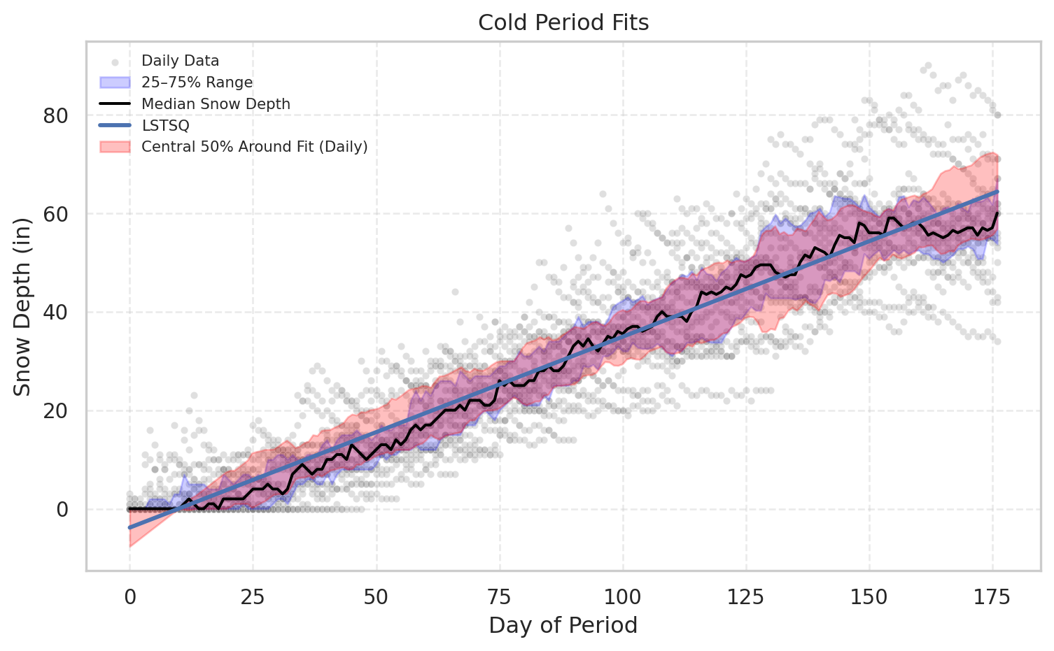
"""
Seaborn-based plot with a *daily symmetric central-50% band* around each fit:
for each day-of-period, compute c(day) = median(|residual|) and plot y_fit ± c(day).
This yields ~half of the data around the fit line for each day.
"""
in_col, day_col = f"{period_name}_InPeriod", f"{period_name}_Day"
df_period = df[df[in_col] & df[day_col].notna()].copy()
if df_period.empty:
print(f"No data found for period '{period_name}'")
return {}
X = df_period[day_col].values
y = df_period["SnowDepth"].values
# --- Median & Quartiles (for context background band) ---
q25 = df_period.groupby(day_col)["SnowDepth"].quantile(0.25)
q75 = df_period.groupby(day_col)["SnowDepth"].quantile(0.75)
med = df_period.groupby(day_col)["SnowDepth"].median()
median_df = pd.DataFrame({day_col: med.index, "q25": q25.values, "q75": q75.values, "median": med.values})
X_med, y_med = median_df[day_col].values, median_df["median"].values
# --- Plot setup ---
plt.figure(figsize=(8, 5))
sns.set_theme(style="whitegrid")
sns.scatterplot(data=df_period, x=day_col, y="SnowDepth",
color="gray", alpha=0.25, s=15, label="Daily Data")
if show_bands:
plt.fill_between(median_df[day_col], median_df["q25"], median_df["q75"],
color="blue", alpha=0.2, label="25–75% Range")
plt.plot(median_df[day_col], median_df["median"],
color="black", linewidth=1.5, label="Median Snow Depth")
# --- Fit lines & metrics ---
metrics = {}
x_fit = np.linspace(X.min(), X.max(), 200)
for i, f in enumerate(fit_functions):
label = labels[i] if labels and i < len(labels) else f"Model {i+1}"
y_pred_full = f(X)
y_pred_med = f(X_med)
y_fit = f(x_fit)
# --- Metrics ---
def _metrics(y_true, y_pred):
ss_res = np.sum((y_true - y_pred) ** 2)
ss_tot = np.sum((y_true - np.mean(y_true)) ** 2)
r2 = 1 - ss_res / ss_tot if ss_tot != 0 else np.nan
rmse = np.sqrt(np.mean((y_true - y_pred) ** 2))
mae = np.mean(np.abs(y_true - y_pred))
return r2, rmse, mae
r2_full, rmse_full, mae_full = _metrics(y, y_pred_full)
r2_med, rmse_med, mae_med = _metrics(y_med, y_pred_med)
metrics[label] = {
"Full": {"R2": r2_full, "RMSE": rmse_full, "MAE": mae_full},
"Median": {"R2": r2_med, "RMSE": rmse_med, "MAE": mae_med},
}
plt.plot(x_fit, y_fit, lw=2.2, label=f"{label}")
# --- Daily symmetric central-50% band around the fit ---
if show_bands:
df_fit = df_period.copy()
df_fit["Residual"] = df_fit["SnowDepth"] - f(df_fit[day_col])
# For each day: c(day) = median(|residual|)
mad50 = (
df_fit.assign(abs_res=lambda d: np.abs(d["Residual"]))
.groupby(day_col)["abs_res"]
.quantile(0.5) # 50th percentile of |residual|
.reset_index()
.rename(columns={"abs_res": "c"})
)
# Interpolate c(day) over x_fit for smooth band
c_interp = np.interp(x_fit, mad50[day_col], mad50["c"])
# Symmetric band: y_fit ± c(day)
plt.fill_between(
x_fit, y_fit - c_interp, y_fit + c_interp,
color="red", alpha=0.25,
label=None if i > 0 else "Central 50% Around Fit (Daily)"
)
plt.xlabel("Day of Period")
plt.ylabel("Snow Depth (in)")
plt.title(title or f"{period_name} Period Fits")
plt.legend(frameon=False, fontsize=8)
plt.grid(True, linestyle="--", alpha=0.4)
plt.tight_layout()
plt.show()
return metrics
def forward_substitution(L, b):
"""
Solve L y = b for y, where L is lower-triangular.
Parameters
----------
L : (n, n) array_like
Lower-triangular matrix.
b : (n,) array_like
Right-hand side vector.
Returns
-------
y : ndarray
Solution vector satisfying L y = b.
"""
L = np.asarray(L, dtype=float)
b = np.asarray(b, dtype=float)
n = L.shape[0]
y = np.zeros_like(b)
for i in range(n):
y[i] = (b[i] - np.dot(L[i, :i], y[:i])) / L[i, i]
return y
def backward_substitution(U, y):
"""
Solve U x = y for x, where U is upper-triangular.
Parameters
----------
U : (n, n) array_like
Upper-triangular matrix.
y : (n,) array_like
Right-hand side vector.
Returns
-------
x : ndarray
Solution vector satisfying U x = y.
"""
U = np.asarray(U, dtype=float)
y = np.asarray(y, dtype=float)
n = U.shape[0]
x = np.zeros_like(y)
for i in range(n - 1, -1, -1):
x[i] = (y[i] - np.dot(U[i, i + 1:], x[i + 1:])) / U[i, i]
return x
# Load Data Set
df = pd.read_csv('data/combined_snowdepth.csv', parse_dates=['Date'])
df['Month'] = df['Date'].dt.month
df['Year']  = df['Date'].dt.year
df['DayOfYear'] = df['Date'].dt.dayofyear

# Compute median snow depth by day of year
median_by_day = df.groupby('DayOfYear')['SnowDepth'].median().rename('MedianSnowDepth')
df = df.merge(median_by_day, on='DayOfYear', how='left')

plot_snowdepth_shifted(df)
# By day-of-year
df = add_period(df, 'Cold', 274, 85)
df = add_period(df, 'Melt', 86, 165)
def build_normal_equations(df, period_name, center=True):

    # Get data
    X, y, empty_model = get_period_data(df, period_name)

    # Convert to numeric arrays
    X = np.asarray(X, dtype=float).ravel()
    y = np.asarray(y, dtype=float).ravel()

    # Center
    X_mean = np.mean(X) if center else 0.0
    x = X - X_mean

    # Linear design matrix: [1, x]
    A = np.column_stack((np.ones_like(x), x))

    # Normal equations
    ATA = A.T @ A
    ATy = A.T @ y

    return ATA, ATy, X_mean, A, y
def solve_cholesky(df, period_name, centered=True):
    # Build normal equations
    ATA, ATy, X_mean, A, y = build_normal_equations(df, period_name, center=centered)
    if ATA is None:
        return np.array([np.nan, np.nan]), np.nan, np.nan

    cond_number = cond(ATA)

    # Cholesky decomposition
    L = cholesky(ATA)

    # Solve via substitution
    y_temp = forward_substitution(L, ATy)
    coeffs = backward_substitution(L.T, y_temp)

    return coeffs, cond_number, X_mean
def solve_qr(df, period_name, centered=True):

    # Build normal equations (gets design matrix + mean)
    ATA, ATy, X_mean, A, y = build_normal_equations(df, period_name, center=centered)
    if ATA is None:
        return np.array([np.nan, np.nan]), np.nan, np.nan

    # QR decomposition (A = Q R)
    Q, R = np.linalg.qr(A)

    # Solve R β = Qᵀ y
    Qt_y = Q.T @ y
    coeffs = backward_substitution(R, Qt_y)

    # Condition number from R
    cond_number = np.linalg.cond(R)

    return coeffs, cond_number, X_mean
def solve_lstsq(df, period_name, centered=True):

    # Build design matrix and vectors
    ATA, ATy, X_mean, A, y = build_normal_equations(df, period_name, center=centered)

    # Solve using NumPy's least-squares
    coeffs, _, _, _ = lstsq(A, y, rcond=None)

    # Compute condition number
    cond_number = np.linalg.cond(A)

    return coeffs, cond_number, X_mean
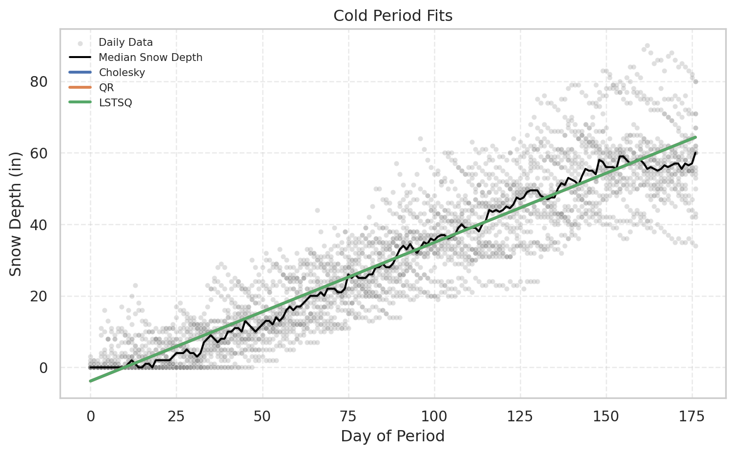
# Build predictor functions
f_chol = make_line_model(chol_coeffs, chol_mean)
f_qr   = make_line_model(qr_coeffs, qr_mean)
f_ls   = make_line_model(lstsq_coeffs, lstsq_mean)

# Plot all together
m = plot_period_fits(df, "Cold", [f_chol, f_qr, f_ls], ["Cholesky", "QR", "LSTSQ"])
def make_polyfit_model(df, period_name, degree=2):

    # Get X and y
    X, y, empty_model = get_period_data(df, period_name)

    # Fit polynomial
    coeffs = np.polyfit(X, y, degree)

    # Predictor function
    model = lambda x_new: np.polyval(coeffs, np.asarray(x_new, dtype=float))

    return model
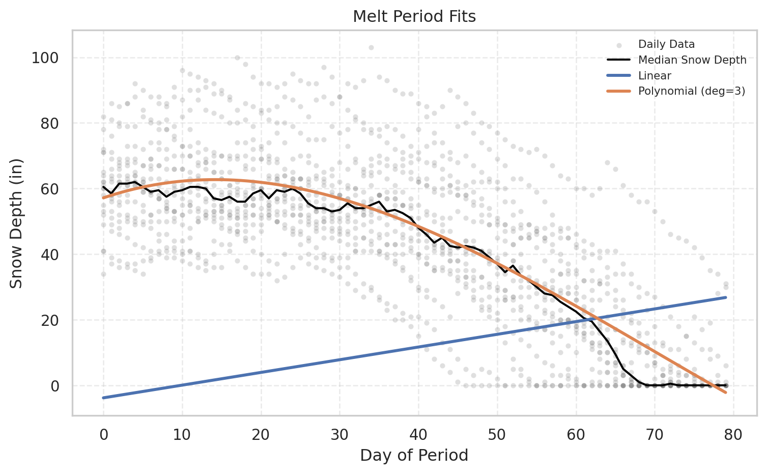
# Fit the linear model for melt
melt_coeffs, _, melt_mean = solve_lstsq(df, 'Cold')
f_lin_melt = make_line_model(melt_coeffs, melt_mean)
# Fit polynomial model for melt
f_poly_melt = make_polyfit_model(df, "Melt", degree=3)

# Plot
melt_poly_metrics = plot_period_fits(df, "Melt", [f_lin_melt,f_poly_melt], ["Linear", "Polynomial (deg=3)"])
cold_metrics=plot_period_fits(df, "Cold", [f_ls], ["LSTSQ"], show_bands=True)
pd.concat({k: pd.DataFrame(v) for k, v in cold_metrics.items()}, axis=1).round(3)
#| echo: False
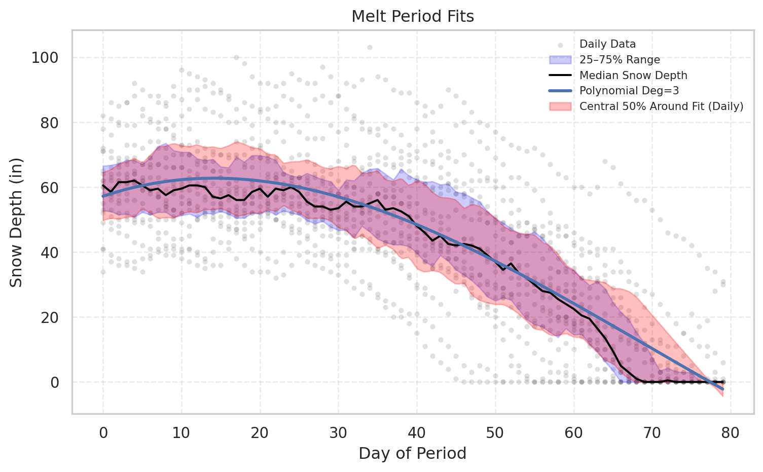
melt_metrics=plot_period_fits(df, "Melt", [f_poly_melt], ["Polynomial Deg=3"], show_bands=True)
#import pandas as pd
pd.concat({k: pd.DataFrame(v) for k, v in melt_metrics.items()}, axis=1).round(3)